Model finding¶

The Alloy Analyzer relies on a procedure called model finding to execute the analysis commands. This procedure, in turn, relies on off-the-shelf solvers for Boolean satisfiability problems (SAT). This topic provides an overview of this process, pointing out to other references for more detailed presentations.

Relational model finding¶

The Analyzer relies on an intermediate tool to perform relational model finding named Kodkod [FSE04]. Kodkod is also based on first-order relational logic, but is stripped of all the structure and syntactic sugar supported by the Alloy language: a Kodkod problem is simply a set of relations bounded by tuple sets and a single formula that will be tested for satifiability. Relations have both a lower-bound declaring which tuples it must contain, and an upper-bound declaring which tuples it may contain. These bounds allow the user to express some partial-knowledge about the possible solutions to the problem. If a Kodkod problem is satisfiable, an instance is returned that assigns a tuple set to each declared relation, ensuring each tuple set is within the specified bounds. The problem’s relations are derived from the signatures and fields declared in the Alloy model, and their bounds from the scope of the command under analysis. The problem’s formula contains the model facts and constraints defined in the command, as well as additional restrictions to encode the signature hierarchy and multiplicity constraints. For check commands, the expected property is negated so that Kodkod will search for counter-examples, i.e., instances that obey all the model’s constraints but break the expected property. Kodkod is also responsible for performing Skolemization (see below), and detecting and enforcing symmetry breaking.

Let us get back to our file system example from the Structural modeling chapter, and consider the following simple command with a small scope, asking for instances where all entries point to directories.

run all_entries_dir {
  Entry.object in Dir
} for 2

Given this scope, a universe with 6 atoms is created, with 2 atoms for each top-level signature. Then the following relations, and the respective lower- and upper-bounds, are declared in the Kodkod problem .

Root    = {(Root0)} {(Root0)}
Dir$    = {}        {(Object0)}
File    = {}        {(Object0)}
Entry   = {}        {(Entry0),(Entry1)}
Name    = {}        {(Name0),(Name1)}

entries = {}        {(Root0,Entry0),(Root0,Entry1),(Object0,Entry0),(Object0,Entry1)}
object  = {}        {(Entry0,Root0),(Entry1,Root0),(Entry0,Object0),(Entry1,Object0)}
name    = {}        {(Entry0,Name0),(Entry1,Name1),(Entry0,Name1),(Entry0,Name1)}

Note that there isn’t a relation created for signatures that are extended by others. Instead, whenever called, they are replaced by the union of all its children signatures. If the signature is not abstract, then a new relation is declared to encode the atoms that do not belong to any of its children (we denote this set with a $ suffix). For instance, any call to Dir in an expression is replaced by Root + Dir$ in Kodkod, and calls to Object by File + Root + Dir$ (since Object is abstract, there are no objects that are not files or directories). Note also that, since Root has multiplicity one, its lower-bound is the same as its upper-bound, making its bounds exact; all other relations in this model have an empty lower-bound.

Then, besides the constraints imposed by the model’s facts and the run command, a few other constraints are introduced from the signature declarations. The first, shown below, forces the set of directories and files to be disjoint.

no (Root + Dir$) & File

The others enforce the type and multiplicity of the binary relations. Below are the constraints corresponding to the object relation. The first constraint enforces the multiplicity one for all entries and the appropriate range type, Object. The second constraint enforces the type of the domain, Entry. These constraints may seem a bit spurious when looking at the upper-bound of object, since it only contains pairs relating entries and objects. However, recall that at this point it is still unknown which atoms will effectively exist in the instance. For instance, Entry can even be empty, and object must be restricted accordingly during solving.

all e : Entry | one e.object and e.object in Root + Dir$ + File
object.univ in Entry

You can actually inspect the generated Kodkod problem by setting menu option Options ‣ Record the Kodkod input/output to Yes. When turned on, words Assertion or Predicate in the Analyzer log, for check and run commands respectively, will open a pop-window with this information. Below is how it looks for the command above.

You can inspect the full formula that was extracted from an Alloy model after all the structure was flattened (it will probably be a bit more verbose than the simplified snippets shown above). You’ll also find the corresponding Java code that allows the generation of that problem, since Kodkod does not support a concrete syntax for defining problems.

Alloy model

Full model for the section

Download and explore the files relevant for the model at this point of the book.

From relational logic to SAT¶

Kodkod relies on off-the-shelf SAT solvers to solve model finding problems. SAT solvers process only propositional formulas in conjunctive normal form (CNF), and generating these from complex Kodkod problems is not trivial [FSE04]. Roughly, if the universe has u atoms, each n-ary relation is seen as an n-dimensional Boolean matrix with size u, where each entry in the matrix denotes whether an n-ary tuple belongs to the relation. Using the bounds declared for the relation, some of these entries will be necessarily true, and some necessarily false; for those whose value is not pre-defined in the bounds, Boolean variables are created whose value will be determined by the solver. Then, relational operations are converted into corresponding matrix operators. For instance, the union + is encoded as entrywise matrix disjunction, while composition . is encoded as matrix multiplication. Atomic formulas are converted accordingly. For instance, inclusion in is encoded as the conjunction of entrywise implications. Finally, first-order operators are translated into propositional logic, which is possible because at this point the finite universe of atoms is known. So universal quantifications all are flattened into conjunctions and existential some into disjunctions.

Let us get back to our example. It has 6 atoms, so unary relations are represented by 6 x 1 matrices (a vector). Below are the matrices corresponding to the unary relations. Notice how tuples that necessarily belong to a relation due to its lower-bound are set to true (here only Root), and those outside the upper-bound are set to false. Those between the lower- and upper-bound are assigned a new Boolean variable.

Root

Dir$

File

Entry

Name

Root0

$\top$

Root0

$\bot$

Root0

$\bot$

Root0

$\bot$

Root0

$\bot$

Object0

$\bot$

Object0

$v_1$

Object0

$v_2$

Object0

$\bot$

Object0

$\bot$

Entry0

$\bot$

Entry0

$\bot$

Entry0

$\bot$

Entry0

$v_3$

Entry0

$\bot$

Entry1

$\bot$

Entry1

$\bot$

Entry1

$\bot$

Entry1

$v_4$

Entry1

$\bot$

Name0

$\bot$

Name0

$\bot$

Name0

$\bot$

Name0

$\bot$

Name0

$v_5$

Name1

$\bot$

Name1

$\bot$

Name1

$\bot$

Name1

$\bot$

Name1

$v_6$

Getting back to command all_entries_dir, relation Root + Dir$ (i.e., relation Dir) is calculated by the entrywise disjunction of the corresponding matrices, resulting in the matrix below.

`Root + Dir$`
`Root0`	$\top$
`Object0`	$v_1$
`Entry0`	$\bot$
`Entry1`	$\bot$
`Name0`	$\bot$
`Name1`	$\bot$

The binary relations are represented by 6 x 6 matrices. Below is the matrix for object (matrices for entries and name are omitted but look similar).

`object`	`Root0`	`Object0`	`Entry0`	`Entry1`	`Name0`	`Name1`
`Root0`	$\bot$	$\bot$	$\bot$	$\bot$	$\bot$	$\bot$
`Object0`	$\bot$	$\bot$	$\bot$	$\bot$	$\bot$	$\bot$
`Entry0`	$v_{7}$	$v_{8}$	$\bot$	$\bot$	$\bot$	$\bot$
`Entry1`	$v_{9}$	$v_{10}$	$\bot$	$\bot$	$\bot$	$\bot$
`Name0`	$\bot$	$\bot$	$\bot$	$\bot$	$\bot$	$\bot$
`Name1`	$\bot$	$\bot$	$\bot$	$\bot$	$\bot$	$\bot$

Continuing with command all_entries_dir, we must calculate composition Entry.object, which is encoded as matrix multiplication. The result is the following vector. Intuitively, this states that, for instance, atom Object0 is present in Entry.object if Entry0 exists in Entry ($v_3$) and object relates those two atoms ($v_9$), or Entry1 exists in Entry ($v_4$) and is related with Object0 through object ($v_{10}$).

`Entry.object`
`Root`	$(v_3 \wedge v_7) \vee (v_4 \wedge v_8)$
`Object`	$(v_3 \wedge v_9) \vee (v_4 \wedge v_{10})$
`Entry0`	$\bot$
`Entry1`	$\bot$
`Name0`	$\bot$
`Name1`	$\bot$

Now, it only remains to encode the inclusion Entry.object in Dir through entrywise implication of the two corresponding matrices. The result is the following propositional formula.

\[\begin{split}&(((v_3 \wedge v_7) \vee (v_4 \wedge v_8)) \rightarrow \top) \wedge (((v_3 \wedge v_9) \vee (v_4 \wedge v_{10})) \rightarrow v_1) \\ &\equiv \\ &((v_3 \wedge v_9) \vee (v_4 \wedge v_{10})) \rightarrow v_1\end{split}\]

This reads as: if atom Object0 belongs to Entry.object, then it must belong to Dir$ ($v_1$). The first conjunct was trivially true since it related to Root0, which is necessarily in Dir through Root. Although we avoided it for simplicity, in practice, the resulting formula will be in CNF.

When the Analyzer reports the result of a command, you can actually get a bit of an insight of the complexity of the SAT problem deployed underneath. The primary vars reported are precisely those that correspond to tuples of the problem’s relations. The execution of command all_entries_dir shown above reported 18 primary variables (the 10 shown above plus another 8 for the omitted entries and name relations). The vars and clauses result from the translation of the problem’s formula into CNF.

Since this procedure generates SAT problems, we can then use many different solvers to check satisfiability, and the Analyzer comes packaged with many state-of-the-art SAT solvers. The SAT solver used by Kodkod can be set through the menu option Options ‣ Solver of the Analyzer. By default, this solver is set to SAT4J, a Java SAT solver that is guaranteed to run in every operating system that the Analyzer also runs. While it’s impossible to predict which SAT solver will perform best for each particular model, SAT4J is rarely the fastest, and the user can explore other solvers that come pre-packaged with the Analyzer depending on the operating system, such as Glucose or MiniSAT. Note that instance iteration requires the usage of an incremental SAT solver to be feasible. So if you select a SAT solver that is not incremental (such as Lingeling), you’ll get an error message when trying to iterate instances in the visualizer. Note also that the order on which the instances are generated my change depending on the selected solver (although eventually they will all generate the same set of instances).

Alloy model

Full model for the section

Download and explore the files relevant for the model at this point of the book.

Skolemization¶

Before deploying the solver, Kodkod performs a process called Skolemization whenever outermost existential quantifications occur in run commands (or universal quantifications for check commands). Instead of flattening the existential quantifier to a disjunction, skolemization transforms the problem to a equisatisfiable one, by creating a new free singleton set (a unary relation) for the existentially quantified variable, and then removing the quantifier and leaving just the quantified formula. The solver will then try to search for a value for the new free variable that satisfies the formula. This largely improves the efficiency of the analysis procedures, and as a side-effect such singleton sets are now also part of the generated instance. Moreover, Skolemization allows the analysis of some commands with higher-order quantifications, which is forbidden in Alloy in general. In particular an existential quantified higher-order variable in a run command will be Skolomized to a new relation with the appropriate arity. Such Skolemized variables can be treated as any other relation in the theme customization. You can control how deep the Analyzer will search for quantifications to Skolemize through menu option Options ‣ Skolem depth, but you cannot actually turn it off altogether.

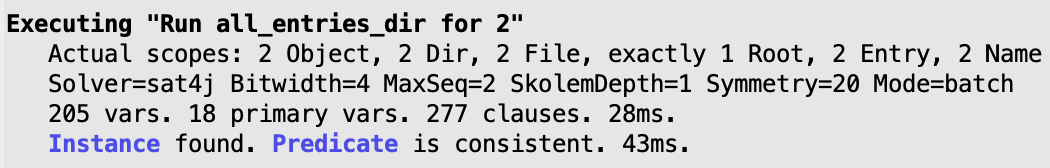
Let us consider an example, for our file system model. For instance, the following command asks for instances where some entry points to a directory.

run some_entries_dir {
  some d : Dir | d in Entry.object
} for 2

The resulting instance is the following, where variable d was Skolemized and is treated as a regular subset of Dir. Its name is prefixed with the command name, and with a $ to distinguish it from the model’s relations. So it appears in the visualization, can be customized in the theme, or called in the evaluator. Here, we just set its border to be Bold. If you look at the log, you’ll notice that the Analyzer now reported 20 primary variables rather than the expected 18: that’s because d was encoded as a relation of the Kodkod problem.

As an example of a higher-order quantification, let’s suppose we wanted to check the obviously false property that all subsets of entries in a file system have the same name. The check command to do so is the following.

check all_entries_same_name {
  all s : set Entry | lone s.name
}

When translated to Kodkod the formula in this command will be negated and originate an existential higher-order quantification that searches for any subset of entries with at least two different names, which would be a counter-example to this property. The Skolomized variable will be part of the counter-example instance, as can be seen in the instance below, where $all_entries_same_name_s contains entries with two different names.

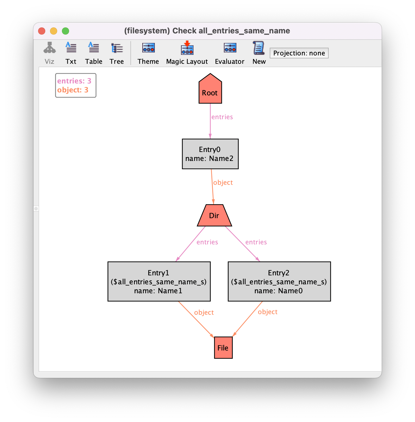
It is worth noting that Skolomization of higher-order quantifications does not add any expressiveness to the language: you could achieve the same result by introducing a new subset signature of Entry and enforcing the same constraints over it (although this would pollute the model, while the higher-order quantification is local to the assertion). If an higher-order quantification cannot be solved by Skolemized an error is thrown by the Analyzer.

Alloy model

Full model for the section

Download and explore the files relevant for the model at this point of the book.

`object`	`Root0`	`Object0`	`Entry0`	`Entry1`	`Name0`	`Name1`
`Root0`	\(\bot\)	\(\bot\)	\(\bot\)	\(\bot\)	\(\bot\)	\(\bot\)
`Object0`	\(\bot\)	\(\bot\)	\(\bot\)	\(\bot\)	\(\bot\)	\(\bot\)
`Entry0`	\(v_{7}\)	\(v_{8}\)	\(\bot\)	\(\bot\)	\(\bot\)	\(\bot\)
`Entry1`	\(v_{9}\)	\(v_{10}\)	\(\bot\)	\(\bot\)	\(\bot\)	\(\bot\)
`Name0`	\(\bot\)	\(\bot\)	\(\bot\)	\(\bot\)	\(\bot\)	\(\bot\)
`Name1`	\(\bot\)	\(\bot\)	\(\bot\)	\(\bot\)	\(\bot\)	\(\bot\)

`Root + Dir$`
`Root0`	\(\top\)
`Object0`	\(v_1\)
`Entry0`	\(\bot\)
`Entry1`	\(\bot\)
`Name0`	\(\bot\)
`Name1`	\(\bot\)

`Entry.object`
`Root`	\((v_3 \wedge v_7) \vee (v_4 \wedge v_8)\)
`Object`	\((v_3 \wedge v_9) \vee (v_4 \wedge v_{10})\)
`Entry0`	\(\bot\)
`Entry1`	\(\bot\)
`Name0`	\(\bot\)
`Name1`	\(\bot\)