A temporal logic primer¶

In chapter Structural modeling, we used relational logic to specify constraints about software structures. As we have seen in the Behavioral modeling chapter, the language also supports temporal logic, to enable the specification of behavioral properties. This topic provides more details about the syntax and semantics of Alloy’s temporal logic.

Everything is a trace¶

What do we mean by “the behaviors of the system”? In Alloy, we view a system as the set of all its execution traces, and every such trace is a feasible infinite sequence of states of the system. Here, “feasible” means that each trace much follow the constraints of the model. The constraints of the model include the Alloy facts and the constraints that are included in the signature declarations, such as the multiplicity constraints. In each state, a relational value is associated with each declared signature and field. If a signature or field is declared as mutable, that its value can change along the trace. Be aware that if a top-level signature is declared as mutable then relations univ and iden will also be mutable, since univ is the union of all top-level sigs, and iden is the identity relation over univ.

Let us consider for instance the following trace of our file sharing web app.

In this scenario, which we will use as an illustrating example in this topic, there are two files and two tokens. A file is depicted in red if it is shared. Tokens are not represented in the picture.

Let us define this scenario in Alloy terms. The set of atoms (the universe) consists of the two files and the two tokens, which are named after their signature name by Alloy: File0, File1, Token0, Token1. Alloy Analyzer produces the following depiction for this scenario. We use here the same visualization theme as in chapter Behavioral modeling: the files are depicted as circles and the tokens as grey rectangles, the files that are not currently uploaded are in white, the uploaded ones are in yellow, the trashed ones are in red. When inspecting a trace, the visualizer starts by focusing on the first two states of a trace (state 0 and state 1).

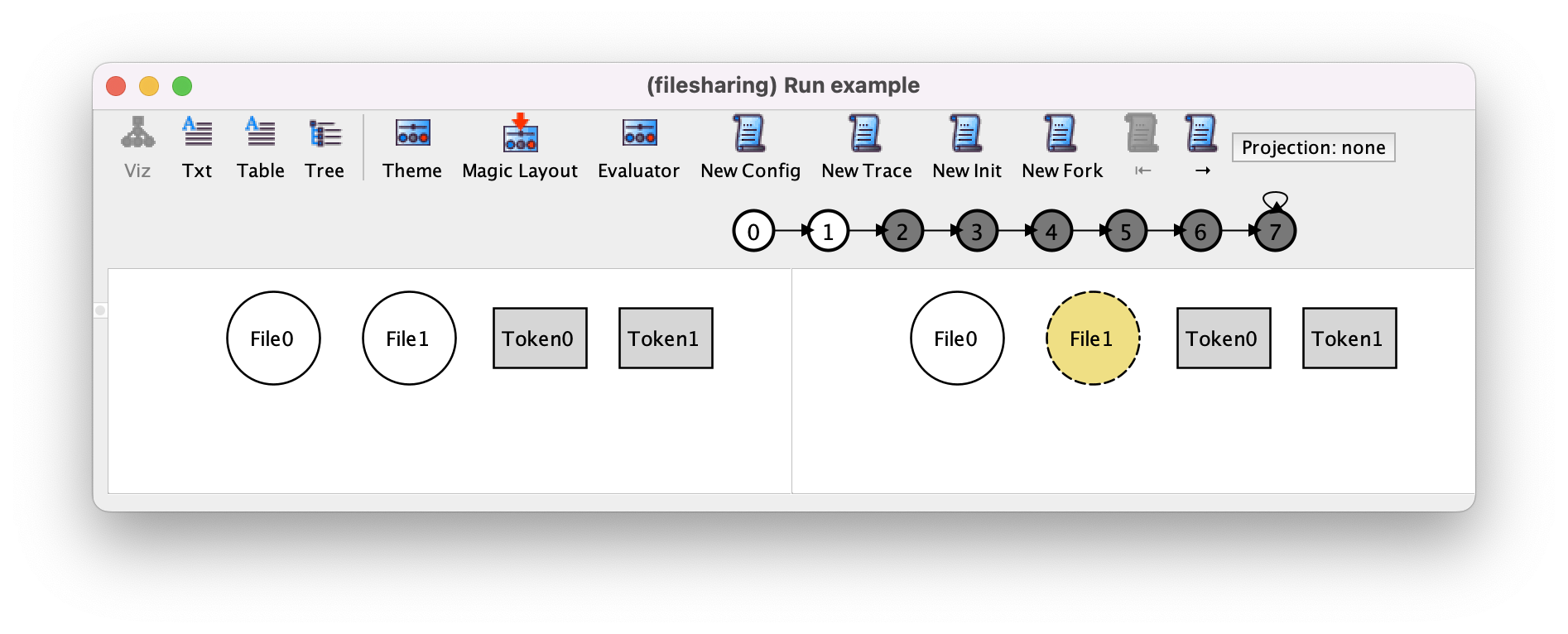
All along the trace, the signatures File and Token have a constant value (because they are static signatures), which is the following.

File  = {(File0),(File1)}
Token = {(Token0),(Token1)}

Now, if we look at the content of the first two states, we see that

in the initial state, the signatures uploaded, trashed and the field shared are empty,
in the second state, uploaded = {(File1)}, and trashed and shared are still empty.

By pressing pressing → a couple of times we can focus on the 3rd and 4th states (state 2 and state 3) of the trace, corresponding to the transition where one file is shared.

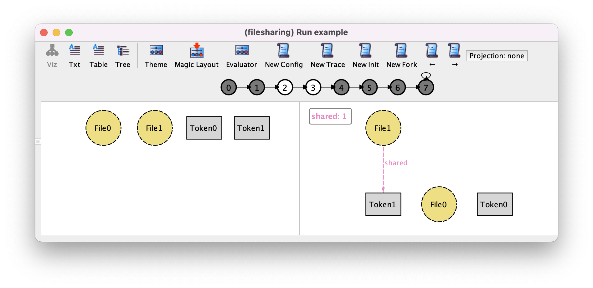
We can see that in state 2 (left-hand side) shared is empty and that uploaded = {(File0),(File1)}, and that in state 3 (right-hand side) shared = {(File1,Token1)}.

In the following, we will use this scenario to illustrate the semantics of temporal connectives.

Temporal connectives¶

The constraints of the model are expressed in Alloy’s logic, which combines relational logic and Linear Temporal Logic (LTL) [FOCS77]. The logic that results from this combination is named Relational Linear Temporal Logic (RLTL). The temporal logic connectives supported by Alloy are the following.

Future-time connectives	Past-time connectives
`after`	`before`
`eventually`	`once`
`always`	`historically`
`until`	`since`
`releases`	`triggered`

The informal meaning of the future-time connectives is the following.

Connective	Informal meaning
`after P`	`P` is true in the next state
`eventually P`	`P` is true in a future state
`always P`	`P` is true in all future states
`P until Q`	`Q` is true in a future states and `P` is true until then
`P releases Q`	`Q` can only stop being true after `P` is true

To be more precise, a temporal logic formula is interpreted in a given state of a trace. Given a trace \(\tau\) the interpretation of every connective is given the state of index \(i ≥ 0\). Given a formula P we write \(\tau,i \models\) P to denote the fact that P is true in the state \(i\) of \(\tau\). We consider that a trace \(\tau\) satisfies a formula P, denoted \(\tau \models\) P, if P is true in its first state, that is \(\tau,0 \models\) P. And a formula is valid in a model if it is valid in all feasible traces of the model.

The following table shows the formal semantics of the future-time connectives.

Connective	Formal meaning
\(\tau,i \models\) `after P`	\(\tau,i+1 \models\) `P`
\(\tau,i \models\) `eventually P`	\(\exists j \ge i \cdot \tau,j \models\) `P`
\(\tau,i \models\) `always P`	\(\forall j \ge i \cdot \tau,j \models\) `P`
\(\tau,i \models\) `P until Q`	\(\exists j \ge i \cdot \tau,j \models\) `Q` \(\wedge\) \(\forall i \le k < j \cdot \tau,k \models\) `P`
\(\tau,i \models\) `P releases Q`	\(\exists j \ge i \cdot \tau,j \models\) `P` \(\wedge\) \(\forall i \le k \le j \cdot \tau,k \models\) `Q` \(\; \vee \;\) \(\forall j \ge i \cdot \tau,j \models\) `Q`

To illustrate the connectives, here are some examples of formulas, which are all valid in the trace that is shown above. Notice that they do not necessarily hold in all the possible traces of the file sharing example.

after some uploaded
eventually some trashed
always (some f : File | upload[f] implies after some uploaded)
(some f : File | upload[f]) until (some f : File, t : Token| share[f, t])
(some f : File | delete[f]) releases no trashed

As in relational logic, some connectives can be defined in terms of others. In particular, it is known that after and until are sufficient to define all other future-time connectives. For example, eventually P is the same as (not P) until P, always P is the same as not eventually not P and P releases Q is the same as not ((not P) until not Q) or the same as (Q until (Q and P)) or always Q.

The informal meaning of the past-time connectives is the following, and it’s dual to the future-time connectives.

Connective	Informal meaning
`before P`	`P` is true in the previous state
`once P`	`P` is true in a past state
`historically P`	`P` is true in all past states
`P since Q`	`Q` is true in a past state and `P` is true since then
`P triggered Q`	`Q` was at least true since `P` was true

The formal semantics of the past-time connectives is given in the following table.

Connective	Formal meaning
\(\tau,i \models\) `before P`	\(i > 0 \wedge \tau,i-1 \models\) `P`
\(\tau,i \models\) `once P`	\(\exists j \le i \cdot \tau,j \models\) `P`
\(\tau,i \models\) `historically P`	\(\forall j \le i \cdot \tau,j \models\) `P`
\(\tau,i \models\) `P since Q`	\(\exists j \le i \cdot \tau,j \models\) `Q` \(\wedge\) \(\forall j < k \le i \cdot \tau,k \models\) `P`
\(\tau,i \models\) `P triggered Q`	\(\exists j \le i \cdot \tau,j \models\) `P` \(\wedge\) \(\forall j \le k \le i \cdot \tau,k \models\) `Q` \(\; \vee \;\) \(\forall j \le i \cdot \tau,j \models\) `Q`

As examples, let us consider the following formulas, which hold in the 4th state of our illustrating scenario. Again, they do not necessarily hold in other states of the trace nor in other traces of the file sharing model.

some shared and before no shared
once no uploaded
some t : token | historically t not in File.shared
File = uploaded since some f : File | upload[f]
(some f : File | upload[f]) triggered after some uploaded

As we said above, we consider that a trace satisfies a formula if its initial state satisfies it. A practical consequence is that a formula in Alloy (whether it is a fact or a property in a check or run command) is interpreted in the initial state of a trace. So, past-time connectives only make sense if they appear in the scope of future-time connectives. For instance, consider the following formula, meaning that some token has never been used: some t : Token | historically t not in File.shared. Interpreting this formula in the initial state of a trace makes it the same as some t : Token | t not in File.shared, which means that some token is not used, because there are no other states before the initial one. In other words, the past-time connective is useless. However, if historically is in the scope of a future-time connective, such as always, it can be useful. For instance, the formula all f : File, t : Token | always (share[f, t] implies historically t not in File.shared means that each time a file is shared with a token, this token has never been used before. Also, note that before is always false in the first state of the trace.

Expressiveness of linear temporal logic¶

Are past-time connectives really useful? A well-known theoretical result for LTL is that past-time connectives do not add any expressiveness to the logic [POPL80]. In other words, after and until are enough to express any property that is expressible in LTL. However, we also know [EATCS03] that past-time connectives allow for exponentially more succinct formulas, which make them very useful in practice.

What do you mean by temporal? In the literature, there are in fact several kinds of temporal logics. Their purpose is to reason over the behavior of a system, but they differ on all sorts of aspects. In the literature, the temporal logic at work in Alloy is referred to as Linear Temporal Logic (LTL) or sometimes Linear Temporal Logic with Past (PLTL). Although this is probably the most commonly used temporal logic, some kinds of temporal reasoning are not possible with LTL. For instance, if one needs to reason about different possible execution traces, a branching-time temporal logic, such as Computation Tree Logic (CTL) [LP81], must be used instead of a linear-time temporal logic. In order to reason about the amount of time that passed between different states, some other kind of temporal logics, which are called timed logics [LICS90], can also be used.

Why does Alloy only consider infinite traces? There exist some frameworks where the length of traces can be finite, but this makes the meaning of temporal connectives tricky. For instance, what is the meaning of after P in the last state of a finite trace? Defining it as either \(true\) or \(false\) would be sensible [CAV03]. But in any case, the sames choice applies to after not P, and then not after P is not equivalent to after not P, which is admittedly counter-intuitive. A solution to avoid these issues is to consider infinite traces only. Remark that it is easy to simulate a finite behavior with an infinite trace, by considering a self-loop on the last state. This is in particular possible in case the Alloy model includes a stuttering event (see section Stuttering in the Behavioral modeling chapter).

Why does Alloy only show lasso traces? Remark that some infinite traces cannot be represented by lasso traces: consider, for example, a trace where P is true once in the first state, and then twice in the 3rd and 4th states, and then three times, and so on. This trace never reaches a repeating sequence of states. Therefore it cannot be represented by a lasso trace. However, a theoretical result for LTL called the Small Model Property (SMP) [JACM85] states that if a constraint has a trace that satisfies it, then it has a lasso trace that satisfies it. In other words, if there is no lasso trace satisfying a constraint, then there is no trace at all, which makes it is enough to only search for lasso traces in the analysis.

Is the fact constraining the system behavior required to specify a transition system? As it is presented in chapter Behavioral modeling, it is a good practice to specify an Alloy model as a transition system: a constraint (without any temporal connective) corresponds to the initial states and another constraint imposes that one action (or a stuttering step) occurs in every state. However, you can also add arbitrary temporal formulas as constraints of the model. Then, such formulas constrain the whole execution instead of only constraining the initial state and each transition. This can be useful to abstract away the behavior of some part of the model that we do not want to specify in detail as a transition system. This is typically the case of fairness assumptions, such as the one we specified at the end of chapter Behavioral modeling, to specify the fact that the system should empty the trash periodically.